Tanya Khovanova's Math Blog

I stumbled upon a TED-Ed video with a frog puzzle:

You’re stranded in a rainforest, and you’ve eaten a poisonous mushroom. To save your life, you need an antidote excreted by a certain species of frog. Unfortunately, only the female of the species produces the antidote. The male and female frogs occur in equal numbers and look identical. There is no way to distinguish between them except that the male has a distinctive croak. To your left you spot a frog on a tree stump. You hear a croak from a clearing in the opposite direction, where you see two frogs. You can’t tell which one made the sound. You feel yourself starting to lose consciousness, and you realize that you only have time to run in one direction. Which way should you go: to the clearing and lick both frogs or to the tree stump and lick the stump frog?

My first thought was that male frogs croak to attract female frogs. That means the second frog in the clearing is probably an already-attracted female. The fact that the stump frog is not moving means it is male. I was wrong. This puzzle didn’t assume any knowledge of biology. The puzzle assumes that each frog’s gender is independent from other frogs. Thus this puzzle is similar to two-children puzzles that I wrote so much about. I not only blogged about this, but also wrote a paper: Martin Gardner’s Mistake.

As in two-children puzzles, the solution depends on why the frog croaked. It is easy to make a reasonable model here. Suppose the male frog croaks with probability p. Now the puzzle can be solved.

Consider the stump frog before the croaking:

• It is a female with probability 1/2.
• It is a croaking male with probability p/2.
• It is a silent male with probability (1-p)/2.

Consider the two frogs in the clearing before the croaking:

• Both are female with probability 1/4.
• One is a female and another is a croaking male with probability p/2.
• One is a female and another is a silent male with probability (1-p)/2.
• Both are silent males with probability (1-p)²/4.
• Both are croaking males with probability p²/4.
• One is a silent male and another is a croaking male with probability p(1-p)/2.

The probabilities corresponding to our outcome—a non-croaking frog on the stump and one croaking frog in the clearing—are in bold. Given that the stump frog is silent, the probability that it’s a female is 1/(2-p). Simillarly, given that one clearing frog croaked, the probability that one of them is a female is 1/(2-p). The probabilities are the same: it doesn’t matter where you go for the antidote.

The TED-Ed’s puzzle makes the same mistake that is common in the two-children puzzles. I don’t want to repeat their incorrect solution. The TED-Ed’s frog puzzle is wrong.

(The calculation in the second to last paragraph was corrected on Nov 13, 2021.)

I have written ad nauseam about the ambiguity of problems with children. Usually a problem with two children is formulated as follows:

Mr. Smith has two children and at least one of them is a boy. What is the probability that he has two boys?

I don’t want to repeat my arguments for why this problem is ambiguous. Today I want to discuss other problematic assumptions about these problems.

Assumption 1: The probability of a child being a boy is 1/2. We know that this is not the case. Usually boys are born more often than girls. In addition to that, when policy interferes, the numbers can change. When China had their one-child policy, 118 boys were born per 100 girls. That makes a probability of a boy 0.54.

Assumption 2: The gender of one child in a family is independent of the gender of the other children. I am not sure where this assumption comes from, but I easily came up with a list of possible influences on this situation.

• A family can have identical twins.
• Families that adopt children can choose the gender of those kids.
• There are studies showing that people (especially men) can have a genetic predisposition to one gender of their children over the other.
• Sex-selective abortion is possible in many countries.
• In vitro fertilization and artificial insemination can use sex-selection techniques.
• People may reject their newborns based on sex.
• The decision to have a second child depends on the gender of the first child.

I would like to discuss how the last bullet point changes the probabilities in two children problems. Let us consider China. Up to now China had a one-child policy with some exceptions. In some cases if the first child was a girl, the family was allowed a second child. For the sake of argument, imagine a county where people are allowed to have a second child only if the first one is a girl. A family with two boys wouldn’t exist in this county. Thus the probability of having two boys is zero.

I tried to find the data about the distribution of children by gender in multi-children families. I couldn’t find any. I would be curious to know what happens in real life, especially in China.

A long time ago, before anyone ever heard about ultrasound, there was a psychic who could predict the gender of a future child. No one ever filed a complaint against him.

The psychic had a journal in which he wrote the client’s name and the gender of the future child. The beauty of the scam was that what he wrote in the journal was the opposite gender that he had predicted. Whenever a client complained that the gender was wrong, he would show the journal and argue that the client had misunderstood.

Happy clients don’t return to complain.

Oh, the power of conditional probability! It is useful to understand it to run scams or to expose them.

Round 1 of Who Wants to Be a Mathematician had the following math problem:

Bob and Jane have three children. Given that one child is their daughter Mary, what is the probability that Bob and Jane have at least two daughters?

In all such problems we usually make some simplifying assumptions. In this case we assume that gender is binary, the probability of a child being a boy is 1/2, and that identical twins do not exist.

In addition to that, every probability problem needs to specify the distribution of events over which the probability is calculated. This problem doesn’t specify. This is a mistake and a source of confusion. In most problems like this, the assumption is that something is chosen at random. In this type of problem there are two possibilities: a family is chosen at random or a child is chosen at random. And as usual, different choices produce different answers.

The puzzle above is not well-defined, even though this is from a contest run by the American Mathematical Society!

Here are two well-defined versions corresponding to two choices in randomization:

Bob and Jane is a couple picked randomly from couples with three children and at least one daughter. What is the probability that Bob and Jane have at least two daughters?

Mary is a girl picked randomly from a pool of children from families with three children. What is the probability that Mary’s family has at least two daughters?

Now, if you don’t mind, I’m going to throw in my own two cents, that is to say, my own two puzzles.

Harvard researchers study the influence of identical twins on other siblings. For this study they invited random couples with three children, where two of the children are identical twins.

1. Bob and Jane is a couple picked randomly from couples in the study with at least one daughter. What is the probability that Bob and Jane have at least two daughters?
2. Mary is a girl picked randomly from a pool of children participating in the study. What is the probability that Mary’s family has at least two daughters?

I already wrote about the sliding-window variation of the Secretary Problem. In this variation, after interviewing a candidate for the job, you can pick him or any out of w − 1 candidates directly before him. In this case we say that we have a sliding window of size w. The strategy is to skip the first s candidates, then pick the person who is better than anyone else at the very last moment. I suggested this project to RSI and it was picked up by Abijith Krishnan and his mentor Shan-Yuan Ho. They did a good job that resulted in a paper posted at the arXiv.

In the paper they found a recursive formula for the probability of winning. The formula is very complicated and not explicit. They do not discuss the most interesting question for me: what is the advantage of a sliding window? How much better the probability of winning with the window as opposed to the classical case without the window?

Let us start with a window of size 2, and n applicants. We compare two problems with the same stopping point. Consider the moment after the stopping point when we see a candidate who is better than everyone else before. Suppose this happens in position b. Then in the classic problem we chose this candidate. What is the advantage of a window? When will we be better off with the window? We will be better if the candidate at index b is not the best, and the window allows us to actually reach the best. This depends on where the best secretary is, and what happens in between.

If the best secretary is the next, in position b + 1, then the window gives us an advantage. The probability of that is 1/n. Suppose the best candidate is the one after next, in position b + 2. The window gives us an advantage only if the person in position b + 1 is better than the person in position b. What is the probability of that? It is less than 1/2. From a random person the probability of the next one being better is 1/2. But the person in position b is not random, he is better than random, so the probability of getting a person who is even better decreases and is not more than 1/2. That means the sliding window wins in this case with probability not more than 1/2n.

Similarly, if the best candidate is in position b + k, then the sliding window allows us to win if every candidate between b and b + k is better than the previous one. The probability of the candidate being better at every step is not more than 1/2. That means, the total probability of getting to the candidate in position b + k is 1/2^k-1. So our chances to win when the best candidate is at position b + k are not more than 1/2^k-1n. Summing everything up we get an advantage that is at least 1/n and not more than 2/n.

The probability of winning in the classical case is very close to 1/e. Therefore, the probability of winning in the sliding window case, given that the size of the window is 2, is also close to 1/e.

Let us do the same for a window of any small size w. Suppose the best secretary is in the same window as the stopping candidate and after him, that is, the best candidate is among the next w − 1 people. The probability of this is (w − 1)/n. In this case the sliding window always leads to the best person and gives an advantage over the classical case. When else does the sliding window help? Let us divide the rest of the applicants into chunks of size w − 1. Suppose the best applicant is in the chunk number k. For the sliding window to allow us to get to him, the best candidate in every chunk has to be better than the best one in the previous chunk. The probability of that is not more than 1/2^k-1. The probability that we get to this winner is not more that (w-1)/2^k-1n. Summing it all up we get that the advantage of the window of size w is between (w − 1)/n and 2(w − 1)/n.

I love The Secretary Problem. I first heard about it a long time ago with a different narrative. Then it was a problem about the marriage of a princess:

The king announces that it is time for his only daughter to marry. Shortly thereafter 100 suitors line up in a random order behind the castle walls. Each suitor is invited to the throne room in the presence of the princess and the king. At this point, the princess has to either reject the suitor and send him away, or accept the suitor and marry him. If she doesn’t accept anyone from the first 99, she must marry the last one. The princess is very greedy and wants to marry the richest suitor. The moment she sees a suitor, she can estimate his wealth by his clothes and his gifts. What strategy should she use to maximize the probability of marrying the richest person?

The strategy contains two ideas. The first idea is trivial: if the princess looks at a suitor and he is not better than those she saw before, there is no reason to marry him. The second idea is to skip several suitors at the beginning, no matter how rich they might seem. This allows the princess to get a feel for what kinds of suitors are interested in her. Given that we know the strategy, the interesting part now is to find the stopping point: how many suitors exactly does she have to skip? The answer is ⌊N/e⌋. (You might think that this formula is approximate. Surprisingly, it works for almost all small values. I checked the small values and found a discrepancy only for 11 and 30 suitors.)

The problem is called The Secretary Problem, because in one of the set-ups the employer tries to hire a secretary.

In many situations in real life it is a good idea to sample your options. Whether I’m shopping for an apartment or looking for a job, I always remember this problem, which reminds me not to grab the first deal that comes my way.

Mathematically, I try to find variations of the problem that are closer to real life than the classical version. Here’s one of the ideas I had: you can always delay hiring a secretary until you have interviewed several candidates. You can’t wait too long, as that good secretary you interviewed two weeks ago might have already found a job. And of course the king has a small window of time in which he can run out of the castle and persuade a suitor to come back before he saddles up his horse and rides away.

To make the problem mathematical we should fix the window size as an integer w. When you are interviewing the k-th suitor, you are allowed to go w − 1 suitors back. In other words, the latest you can pick the current suitor is after interviewing w − 1 more people. I call this problem: The Secretary Problem with a Sliding Window.

It is easy to extrapolate the standard strategy to the sliding window problem. There is no reason to pick a suitor who is not the best the princess have seen so far. In addition, if she sees the best person, it is better to wait for the last moment to pick him in case someone better appears. So the strategy should be to skip several people at the beginning and then to pick the best suitor at the last moment he is available.

The difficult part after that is to actually calculate the probabilities and find the stopping point. So I suggested this project to RSI 2015. The project was assigned to Abijith Krishnan under the direction of Dr. Shan-Yuan Ho. Abijith is a brilliant and hard-working student. Not only did he (with the help from his mentor) write a formula for the stopping point and winning probabilities during the short length of RSI, he also resolved the case when the goal is to pick one candidate out of the best two.

If you are interested to see what other RSI students did this year, the abstracts are posted here.

* * *

Do you know a statistics joke?
Probably, but it’s mean!

* * *

Twelve different world statisticians studied Russian roulette. Ten of them proved that it is perfectly safe. The other two scientists were unfortunately not able to join the final discussion.

* * *

A statistician bought a new tool that finds correlations between different fields in databases. Hoping for new discoveries he ran his new tool on his large database and found highly correlated events. These are his discoveries:

• The most correlated fields were the title and the gender. If the title is Mr., then the gender is male.
• The children have the same last names as parents.
• The children are much younger than the parents.
• The main cause of divorces is weddings.

* * *

Scientists discovered that the main cause of living ’till old age is an error on the birth certificate.

* * *

Scientists concluded that children do not really use the Internet. This is proven by the fact that the percentage of people saying ‘No’ when asked ‘Are you over 18?’ is close to zero.

* * *

— Please, close the window, it is cold outside.
— Do you think it will get warmer, after I close it?

This story started when my student asked for an explanation for his grade B in linear algebra. He was slightly above average on every exam and the cut-off for an A was the top 50 percent of the class. I wrote a post in which I asked my readers to explain the situation. Here is my explanation.

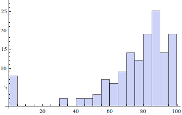
The picture below contains histogram for a typical first midterm linear algebra exam.

The spike in the lowest range indicates zeros for those who missed the exam.

The mean is 74.7 and the median 81.5. As you can see the median is 7 points higher than the mean. That means that if a student performs around average on all the exams, s/he is in the bottom half of the class.

But this is not the whole story. In addition to the above, MIT allows students to drop the class after the second midterm. Suppose 30 students with lower grades drop the class; then the recalculated median for the first midterm for the students who finish the course goes up to 85. This is a difference of more than 10 points from the original average.

If this was a statistics class, then I could have told the puzzled student that he deserves that B. Instead I told him that he didn’t even have the highest score among those with Bs. Somehow that fact made him feel better.

I lead recitations for a Linear Algebra class at MIT. Sometimes my students are disappointed with their grades. The grades are based on the final score, which is calculated by the following formula: 15% for homework, 15% for each of the three midterms, and 40% for the final. After all the scores are calculated, we decide on the cutoffs for A, B, and other grades. Last semester, the first cutoff was unusually low. The top 50% got an A.

Some students who were above average on every exam assumed they would get an A, but nonetheless received a B. The average scores for the three midterm exams and for the final exam were made public, so everyone knew where they stood relative to the average.

The average scores for homework are not publicly available, but they didn’t have much relevance because everyone was close to 100%. However, a hypothetical person who is slightly above average on everything, including the homework, should not expect an A, even if half the class gets an A. There are two different effects that cause this. Can you figure them out?

Here is a setup that works for the several puzzles that follow it:

The sultan decides to test his hundred wizards. Tomorrow at noon he will randomly put a red or a blue hat—from his inexhaustible supply—on every wizard’s head. Each wizard will be able to see every hat but his own. The wizards will not be allowed to exchange any kind of information whatsoever. At the sultan’s signal, each wizard needs to write down the color of his own hat. Every wizard who guesses wrong will be executed. The wizards have one day to decide together on a strategy.

I wrote about puzzles with this setup before in my essay The Wizards’ Hats. My first request had been to maximize the number of wizards who are guaranteed to survive. It is easy to show that you cannot guarantee more than 50 survivors. Indeed, each wizard will be right with probability 0.5. That means whatever the strategy, the expected number of wizards guessing correctly is 50. My second request had been to maximize the probability that all of them will survive. Again, the counting argument shows that this probability can’t be more than 0.5.

Now here are some additional puzzles, including the first two mentioned above, based on the same setup. Suggest a strategy—or prove that it doesn’t exist—in which:

1. 50 wizards will be guaranteed to survive.
2. 100 wizards will survive with probability 0.5.
3. 100 wizards will survive with probability 0.25 and 50 wizards will survive with probability 0.5.
4. 75 wizards will survive with probability 1/2, and 25 wizards survive with probability 1/2.
5. 75 wizards will survive with probability 2/3.
6. The wizards will survive according to a given distribution. For which distributions is it possible?

As I mentioned, I already wrote about the first two questions. Below are the solutions to those questions. If you haven’t seen my post and want to think about it, now is a good time to stop reading.

To guarantee the survival of 50 wizards, designate 50 wizards who will assume that the total number of red hats is odd, and the rest of the wizards will assume that the total number of red hats is even. The total number of red hats is either even or odd, so one of the groups is guaranteed to survive.

To make sure that all of them survive together with probability 0.5, they all need to assume that the total number of red hats is even.