Fair-Share Sequences
Every time I visit Princeton, or otherwise am in the same city as my friend John Conway, I invite him for lunch or dinner. I have this rule for myself: I invite, I pay. If we are in the same place for several meals we alternate paying. Once John Conway complained that our tradition is not fair to me. From time to time we have an odd number of meals per visit and I end up paying more. I do not trust my memory, so I prefer simplicity. I resisted any change to our tradition. We broke the tradition only once, but that is a story for another day.
Let’s discuss the mathematical way of paying for meals. Many people suggest using the Thue-Morse sequence instead of the alternating sequence of taking turns. When you alternate, you use the sequence ABABAB…. If this is the order of paying for things, the sequence gives advantage to the second person. So the suggestion is to take turns taking turns: ABBAABBAABBA…. If you are a nerd like me, you wouldn’t stop here. This new rule can also give a potential advantage to one person, so we should take turns taking turns taking turns. Continuing this to infinity we get the Thue-Morse sequence: ABBABAABBAABABBA… The next 2n letters are generated from the first 2n by swapping A and B. Some even call this sequence a fair-share sequence.
Should I go ahead and implement this sequence each time I cross paths with John Conway? Actually, the fairness of this sequence is overrated. I probably have 2 or 3 meals with John per trip. If I pay first every time, this sequence will give me an advantage. It only makes sense to use it if there is a very long stretch of meals. This could happen, for example, if we end up living in the same city. But in this case, the alternating sequence is not so bad either, and is much simpler.
Many people suggest another use for this sequence. Suppose you are divorcing and dividing a huge pile of your possessions. A wrong way to do it is to take turns. First Alice choses a piece she wants, then Bob, then Alice, and so on. Alice has the advantage as the first person to choose. An alternative suggestion I hear in different places, for example from standupmaths, is to use the Thue-Morse sequence. I don’t like this suggestion either. If Alice and Bob value their stuff differently, there is a better algorithm, called the Knaster inheritance procedure, that allows each of them to think they are getting more than a half. If both of them have the same value for each piece, then the Thue-Morse sequence might not be good either. Suppose one of the pieces they are dividing is worth more than everything else put together. Then the only reasonable way to take turns is ABBBB….
The beauty of the Thue-Morse sequence is that it works very well if there are a lot of items and their consecutive prices form a power function of a small degree k, such as a square or a cube function. After 2k+1 turns made according to this sequence, Alice and Bob will have a tie. You might think that if the sequence of prices doesn’t grow very fast, then using the Thue-Morse sequence is okay.
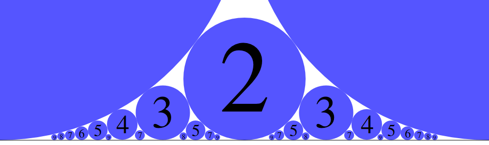
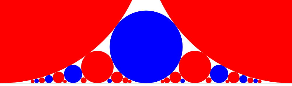
Not so fast. Here is the sequence of prices that I specifically constructed for this purpose: 5,4,4,4,3,3,3,2,2,2,2,1,1,0,0,0. The rule is: every time a turn in the Thue-Morse sequence switches from A to B, the value goes down by 1. Alice gets an extra 1 every time she is in the odd position. This is exactly half of her turns. That is every four turns, she gets an extra 1.
If the prices grow faster than a power, then the sequence doesn’t work either. Suppose your pieces have values that form a Fibonacci sequence. Take a look at what happens after seven turns. Alice will have pieces priced Fn + Fn-3 + Fn-5 + Fn-6. Bob will have Fn-1 + Fn-2 + Fn-4. We see that Alice gets more by Fn-3. This value is bigger than the value of all the leftovers together.
I suggest a different way to divide the Fibonacci-priced possessions. If Alice takes the first piece, then Bob should take two next pieces to tie with Alice. So the sequence might be ABBABBABB…. I can combine this idea with flipping turns. So we start with a triple ABB, then switch to BAA. After that we can continue and flip the whole thing: ABBBAABAAABB. Then we flip the whole thing again. And again and again. At the end we get a sequence that I decided to call the Fibonacci fair-share sequence.
I leave you with an exercise. Describe the Tribonacci fair-share sequence.
Share:
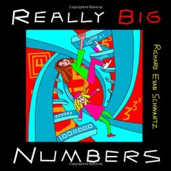 I received a book