Tanya Khovanova's Math Blog

You are given N coins such that two of them are fake and the other coins are genuine. Real coins weigh the same. Fake coins weigh the same and are lighter than real ones. You need to find both fake coins using a balance scale in the smallest number of weighings.

It is easy to estimate the number of weighings from below using information theory. Given N coins you will have N choose 2 different answers. The number of possible answers has to be not more than 3^w, where w is the number of weighings. This generates a trivial information-theoretic bound (ITB) on the number of coins that can be processed in a given number of weighings.

Previous authors used computers to completely analyze small numbers of weighings: from 2 to 5.

My colleagues from Russia, Konstantin Knop and Oleg Polubasov, performed some fantastic programming accompanied with some subtle heuristic and found optimal solutions for up to 10 weighings. For 11 and 12 weighings, the program is not efficient enough to find the optimal solutions: it found some solutions. Surprisingly, for up to 10 weighings, the optimal solutions match the information-theoretic bound (ITB). The results are in the table below. The first row represents the number of weighings w. The second row is the largest number of coins N for which a solution is found. The last row is the information-theoretic bound (ITB) we explained above.

Their paper, Two counterfeit coins revisited, is available in Russian. Lucky for us, 70 of 73 pages are pseudo-code of solutions for which you do not need any Russian. You just need to understand the pseudo-code. Here is the explanation.

Each line begins with its number. After it they have the weighing in the format 1 10 v 4 5 meaning coins 1 and 10 are weighed versus coins 4 and 5. Each weighing is followed by a colon, after which they describe in order actions for three different outcomes of the weighing: equality, the first pan is lighter, and the second pan is lighter. Each action is one of the following:

• => L means go to line L.
• (a, b) means the fake coins are a and b.
• – means this branch is impossible and there is no output.
• => 23. sym indicates the symmetry of the weighing and its result, therefore the resulting go-to line, 23, is omitted as being equivalent to another line.
• – . sym means the output is symmetric to another one.

The line numbers after => in line L are always 3L+1, 3L+2 and 3L+3. The sym symbol implies that line 3L+3 is omitted as a symmetric version of line 3L+2.

For example, here is their solution for 2 weighings and 4 coins in their pseudo-code. An empty line separates different weighings:

0. 1 v 2 : => 1, => 2, => 3. sym

1. 1 v 3 : – , (1, 2), (3, 4).
2. 3 v 4 : – , (1, 3), – . sym

Another solution for 3 weighings and 7 coins:

0. 1 2 v 3 4 : => 1, => 2, => 3. sym

1. 1 v 2 : => 4, => 5, => 6. sym
2. 1 v 2 : (1, 2), => 8, => 9. sym

4. 5 v 6 : (5, 6), (5, 7), – . sym
5. 3 v 4 : – , (1, 3), – . sym
8. 5 v 6 : (1, 7), (1, 5), – . sym

If you want to see an optimal solution for 10 weighings, look at the paper: the algorithm takes 36 pages.

In my paper Nim Fractals written with Joshua Xiong we discovered an interesting graph structure on P-positions of impartial combinatorial games. P-positions are vertices of the graph and two vertices are connected if they are consecutive P-positions in an optimal longest game.

A longest game of Nim is played when exactly one token is removed in each turn. So in Nim two P-positions are connected if it is possible to get from one of them to the other by removing two tokens.

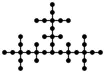
In the paper we discussed the evolution graph of Nim with three piles. The graph has the same structure as three branches of the Ulam-Warburton automaton.

For completeness, I would like to describe the evolution graph of the 2-pile Nim. The P-positions in a 2-pile Nim are pairs (n,n), for any integer n. Two positions (n,n) and (m,m) are connected if and only if m and n differ by 1. The first picture represents this graph.

The Wythoff’s game is more interesting. There are two piles of tokens. In one move a player can take any number of tokens from one pile or the same number of tokens from both piles.

The P-positions (n,m) such that n ≤ m start as: (0,0), (1,2), (3,5), (4,7), (6,10) and so on. They can be enumerated using φ: the golden ratio. Namely, n_k = ⌊kφ⌋ and m_k = ⌊kφ²⌋ = n_k + k, where k ≥ 0.

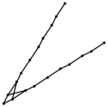
In a longest Wythoff’s game the difference between the coordinates decreases by 1. That is, it takes a maximum of 2k steps to end an optimal game starting from position (n_k,m_k). The picture shows the evolution graph.

The interesting part of the picture is the crossover between two “lines”. From positions with large coordinates like (6,10) with a difference of 4 you can get to only one position with a difference of 3: (4,7) and not (7,4). But from position (3,5) with a difference of 2 you can get to both positions with a difference of 1: (1,2) and (2,1).

I already wrote about the sliding-window variation of the Secretary Problem. In this variation, after interviewing a candidate for the job, you can pick him or any out of w − 1 candidates directly before him. In this case we say that we have a sliding window of size w. The strategy is to skip the first s candidates, then pick the person who is better than anyone else at the very last moment. I suggested this project to RSI and it was picked up by Abijith Krishnan and his mentor Shan-Yuan Ho. They did a good job that resulted in a paper posted at the arXiv.

In the paper they found a recursive formula for the probability of winning. The formula is very complicated and not explicit. They do not discuss the most interesting question for me: what is the advantage of a sliding window? How much better the probability of winning with the window as opposed to the classical case without the window?

Let us start with a window of size 2, and n applicants. We compare two problems with the same stopping point. Consider the moment after the stopping point when we see a candidate who is better than everyone else before. Suppose this happens in position b. Then in the classic problem we chose this candidate. What is the advantage of a window? When will we be better off with the window? We will be better if the candidate at index b is not the best, and the window allows us to actually reach the best. This depends on where the best secretary is, and what happens in between.

If the best secretary is the next, in position b + 1, then the window gives us an advantage. The probability of that is 1/n. Suppose the best candidate is the one after next, in position b + 2. The window gives us an advantage only if the person in position b + 1 is better than the person in position b. What is the probability of that? It is less than 1/2. From a random person the probability of the next one being better is 1/2. But the person in position b is not random, he is better than random, so the probability of getting a person who is even better decreases and is not more than 1/2. That means the sliding window wins in this case with probability not more than 1/2n.

Similarly, if the best candidate is in position b + k, then the sliding window allows us to win if every candidate between b and b + k is better than the previous one. The probability of the candidate being better at every step is not more than 1/2. That means, the total probability of getting to the candidate in position b + k is 1/2^k-1. So our chances to win when the best candidate is at position b + k are not more than 1/2^k-1n. Summing everything up we get an advantage that is at least 1/n and not more than 2/n.

The probability of winning in the classical case is very close to 1/e. Therefore, the probability of winning in the sliding window case, given that the size of the window is 2, is also close to 1/e.

Let us do the same for a window of any small size w. Suppose the best secretary is in the same window as the stopping candidate and after him, that is, the best candidate is among the next w − 1 people. The probability of this is (w − 1)/n. In this case the sliding window always leads to the best person and gives an advantage over the classical case. When else does the sliding window help? Let us divide the rest of the applicants into chunks of size w − 1. Suppose the best applicant is in the chunk number k. For the sliding window to allow us to get to him, the best candidate in every chunk has to be better than the best one in the previous chunk. The probability of that is not more than 1/2^k-1. The probability that we get to this winner is not more that (w-1)/2^k-1n. Summing it all up we get that the advantage of the window of size w is between (w − 1)/n and 2(w − 1)/n.

In my paper with Joshua Xiong on Nim Fractals we explained how to build an evolution graph corresponding to an impartial combinatorial game. The vertices of the graph are P-positions. And two vertices are connected if the two corresponding positions are consecutive P-positions in a longest possible optimal game.

What types of graphs do we get? An evolution graph should have at least one sink: these are our terminal P-positions. Also there are no directed loops: the game is finite. In addition, the distance from a vertex to sinks is uniquely defined: the number of directed edges that is needed to move from this vertex to a sink. This number is equal to half of the number of moves in the longest game, starting from the corresponding P-position.

A natural question arises: Can we build a game from a graph? The graph needs to satisfy the properties above. But other than that, can we? We can consider the graph itself as a game. Players can start at a vertex or an edge. From an edge, they can only move to a vertex where this edge ends. From a vertex they can move to any out-edge. The corresponding evolution graph is the graph itself. Vertices correspond to P-positions and edges to N-positions.

There is an equivalent game with a more uniform description. We put a vertex in the middle of every edge in the evolution graph. The new graph becomes bipartite. Players can start at any vertex. A move is allowed from a vertex following an out-edge to the vertex, where this edge ends. Vertices that are in the same part as terminal positions are P-positions. Other vertices are N-positions.

Without using a calculator, can you tell how much 75² is? If you are reading my blog, with high probability you know that it is 5625. The last two digits of the square of a number ending in 5 are always 25. So we only need to figure out the first two digits. The first two digits equals 7 times 8, or 56, which is the first digit of the original number (7) multiplied by the next number (8).

I was good at mental arithmetic and saved myself a lot of money back in the Soviet Union. Every time I shopped I calculated all the charges as I stood at the cash register. I knew exactly how much to pay, which saved me from cheating cashiers. To simplify my practice, the shelves were empty, so I was never buying too many items.

When I moved to the US, the situation changed. Salespeople are not trying to cheat, not to mention that they use automatic cash registers. In addition, the US sales taxes are confusing. I remember how I bought three identical chocolate bars and the total was not divisible by 3. So I completely dropped my at-the-cash-registers mental training.

Being able to calculate fast was somewhat useful many years ago. But now there is a calculator on every phone.

John H. Conway is a master of mental calculations. He even invented an algorithm to calculate the day of the week for any day. He taught it to me, and I too can easily calculate that July 29 of 1926 was Thursday. This is not useful any more. If I google “what day of the week is July 29, 1926,” the first line in big letters says Thursday.

One day a long time ago I was watching a TV show of a guy performing mental tricks: remembering large numbers, multiplying large numbers, and so on. At the end, to a grand fanfare, he showed his crowned trick. A member from the audience was to write down a 2-digit number, and to raise it to the fifth power using a calculator. The mental guy, once he is told what the fifth power was, struggled with great concentration and announced the original number.

I was so underwhelmed. Anyone knows that the last digit of a number and its fifth power are the same. So he only needs to guess the first digit, which can easily be estimated by the size of the fifth power.

I found the description of this trick online. They recommend memorizing the fifth powers of the numbers from 1 to 9. After that, you do the following. First, listen to the number. Next, the last digit of the number you hear is the same as the last digit of the original number. To figure out the first digit of the original number, remove the last 5 digits of the number you hear. Finally, determine between which fifth powers it fits. This makes sense. Or, you could be lazy and remember only meaningful digits. For example, 39⁵=90,224,199, and 40⁵=102,400,000. So if the number is below 100,000,000, then the first digit is less than 4.

You do not have to remember the complete fifth powers of every digit. You just need to remember significant ranges. Here they are:

Besides, for this trick the guy needed to guess one out of one hundred number. He had a phenomenal memory, so he could easily have remembered one hundred fifth powers. Actually he doesn’t need to remember all the numbers, only the differentiated features. On this note, there is a cool thing you can do. You can guess the number before the whole fifth power is announced. One caveat: a 1-digit number x and 10x when taken to the fifth power, both begin with the same long string of digits. So we can advise the audience not to suggest a 1-digit number or a number divisible by 10, as that is too easy (without telling the real reason).

Now we can match a start of the fifth power to its fifth root. Three first digits are almost always enough. Here is the list of starting digits and their match: (104,16), (107,64), (115,41), (116,65), (118,26), (12,66), (130,42), (135,67), (141,17), (143,27), (145,68), (147,43), (156,69), (161,11), (164,44), (17,28), (180,71), (184,45), (188,18), (19,72), (2051,29), (2059,46), (207,73), (221,74), (229,47), (23,75), (247,19), (248,12), (253,76), (254,48), (270,77), (282,49), (286,31), (288,78), (30,79), (33,32), (345,51), (348,81), (370,82), (371,13), (38,52), (391,33), (393,83), (40,21), (4181,53), (4182,84), (44,85), (454,34), (459,54), (470,86), (498,87), (50,55), (51,22), (525,35), (527,88), (53,14), (550,56), (558,89), (601,57), (604,36), (62,91), (64,23), (656,58), (659,92), (693,37), (695,93), (71,59), (73,94), (75,15), (77,95), (792,38), (796,24), (81,96), (84,61), (85,97), (902,39), (903,98), (91,62), (95,99), (97,25), (99,63).

Or, you can come to the mental guy’s performance and beat him by shouting out the correct answer before he can even finish receiving the last digit. This would be cool and cruel at the same time.

Since I was a child I prided myself on knowing arithmetic. I knew how to add fractions. I knew that 2/3 plus 1/4 is 11/12. Some kids around me were struggling and often summed it up the wrong way by adding numerators and denominators separately and getting 3/7 as a result.

As I grew older I found more reasons to ignore the wrong way. For example, the result of such addition depends on the representation of a fraction, not on the fraction itself, and this was bad.

Oh well. I was growing older, but not wiser. Now mathematicians study this wrong addition of fractions. They call such a sum a mediant of two rational numbers. To avoid the dependency on the representation of fractions, the fractions are assumed to be in the lowest terms.

Let us start with the sequence of fractions: 0/1 and 1/0. This sequence is called the Stern-Brocot sequence of order 0. The Stern-Brocot sequence of order n is generated from the Stern-Brocot sequence of order n − 1 by inserting mediants between consecutive elements of the sequence. For example, the Stern-Brocot sequence of order 2 is 0/1, 1/2, 1/1, 2/1, 1/0.

Where are the trees promised in the title? We can build a portion of this binary tree out of the sequence of order n in the following manner. First, ignore the starting points 0/1 and 1/0. Then assign a vertex to every number in the sequence. After that, connect every mediant to one of the two numbers it was calculated from. More precisely, if a number first appeared in the i-th sequence, its only parent is the number that first appeared in the sequence i−1.

There is beautiful theorem that states that every non-negative rational number appears in the Stern-Brocot sequences. The proof is related to continued fraction. Suppose a rational number r is represented as a continued fraction [a₀;a₁,a₂,…,a_k], where a_k is assumed to be greater than 1 for uniqueness. Then this number first appears in the Stern-Brocot tree of order a₀ + a₁ + a₂ + … + a_k + 1, and its parent is equal [a₀;a₁,a₂,…,a_k − 1].

My PRIMES student, Dhroova Ayilam, was working on a project suggested by Prof. James Propp. The goal was to find out what happens if we start with any two rational numbers in lowest terms. Dhroova proved that as with the classical Stern-Brocot trees, any rational number in a given range appears in the tree. His paper Modified Stern-Brocot Sequences is available at the arXiv.

I mentor three PRIMES projects. One of them, with Joshua Xiong from Acton-Boxborough Regional High School, is devoted to impartial combinatorial games. We recently found a connection between these games and cellular automata. But first I need to remind you of the rules of Nim.

In the game of Nim there are several piles with counters. Two players take turns choosing a pile and removing several counters from it. A player loses when he or she who doesn’t have a turn. Nim is the most famous impartial combinatorial game and its strategy is well known. To win, you need to finish your move in a so called P-position. Nim P-positions are easy to calculate: Bitwise XOR the number of counters in all the piles, and if the result is zero then it’s a P-position.

The total number of counters in a P-position is even. So we calculated the sequence a(n): the number of P-positions in the game of Nim with three piles with the total number of counters equal to 2n. As soon as we got the sequence we plugged it into the OEIS, and voilà it was there: The sequence A130665 described the growth of the three branches of the Ulam-Warburton cellular automaton.

The first picture shows the automaton after 6 generations. The automaton consists of cells that never die and it grows like this: start with a square on a square grid. In the next generation the squares that share exactly one side with the living squares are born. At the end remove the Southern branch.

Everything fell into place. We immediately realized that the language of the automata gives us the right words to describe what we know about the game of Nim.

Now we want to describe the automaton related to any impartial combinatorial game. Again, the cells never die and the initial cells correspond to terminal P-positions. People who write programs for calculating P-positions will find a notion of the next generation very natural. Indeed, the program usually starts with the terminal P-positions: they are generation 0. Then we can proceed by induction. Suppose we have found P-positions up to generation i. Denote the positions that are one move away from generation i and earlier as N_i. Then the P-positions that do not belong to generation i and earlier and from which all moves belong to N_i are the P-positions from generation i + 1.

This description explains the generations, but it doesn’t explain who is the parent of a particular P-position. The parent-child relations are depicted as edges on the cellular automaton graph. The parent of position P₁ from generation i + 1 is a P-position P₂ in generation i that can be reached from P₁ in the game.

The parent-child relationship in the game of Nim is especially easy to explain. A P-position P₁ is a parent of a P-position P₂ if P₁ differs from P₂ in exactly two piles and it has one fewer counter in each of these piles. For example, a P-position (1,3,5,7) has six parents, one of them is (1,3,4,6). In the game with thee piles a P-position always has exactly one parent.

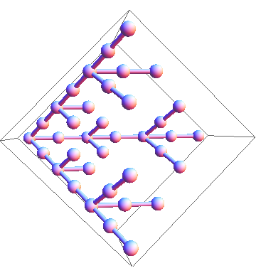
A position in the game of Nim with three piles is naturally depicted as a triple of numbers, that is as a point in 3D. The picture below shows the Nim automaton in 3D at generation 6.

Our paper, Nim Fractals, about sequences enumerating P-positions and describing the automaton connection in more detail is posted at the arXiv:1405.5942. We give a different, but equivalent definition of a parent-child relationship there. A P-position P₁ is a parent of P₂ if there exists an optimal game such that P₁ is achieved from P₂ in exactly two moves in a game which takes the longest number of possible moves.

This is one of my favorite jokes:

Three logicians walk into a bar. The waitress asks, “Do you all want beer?”
The first logician answers, “I do not know.”
The second logician answers, “I do not know.”
The third logician answers, “Yes.”

This joke reminds me of hat puzzles. In the joke each logician knows whether or not s/he wants a beer, but doesn’t know what the others want to drink. In hat puzzles logicians know the colors of the hats on others’ heads, but not the color of their own hats.

This is a hat puzzle which has the same answers as in the beer joke. Three logicians walk into a bar. They know that the hats were placed on their heads from the set of hats below. The total number of available red hats was three, and the total number of available blue hats was two.

Three logicians walk into a bar. The waitress asks, “Do you know the color of your own hat?'”
The first logician answers, “I do not know.”
The second logician answers, “I do not know.”
The third logician answers, “Yes.”

The puzzle is, what is the color of the third logician’s hat?

This process of converting jokes to puzzles reminds me of the Langland’s Program, which tries to unite different parts of mathematics. I would like to unite jokes and puzzles. So here I announce my own program:

Tanya’s Program: Find a way to convert jokes into puzzles and puzzles into jokes.

I submitted four papers to the arXiv this Spring. Since then I wrote four more papers:

• (with Leigh Marie Braswell) Cookie Monster Devours Naccis. History and Overview arXiv: arXiv 1305.4305.

  In 2002, Cookie Monster appeared in The Inquisitive Problem Solver. The hungry monster wants to empty a set of jars filled with various numbers of cookies. On each of his moves, he may choose any subset of jars and take the same number of cookies from each of those jars. The Cookie Monster number is the minimum number of moves Cookie Monster must use to empty all of the jars. This number depends on the initial distribution of cookies in the jars. We discuss bounds of the Cookie Monster number and explicitly find the Cookie Monster number for Fibonacci, Tribonacci and other nacci sequences.

• A Line of Sages.
  • PDF.

  A new variation of an old hat puzzle, where sages are standing in line one behind the other.

• (Jesse Geneson and Jonathan Tidor) Convex geometric (k+2)-quasiplanar representations of semi-bar k-visibility graphs. Combinatorics arXiv: arXiv 1307.1169.

  We examine semi-bar visibility graphs in the plane and on a cylinder in which sightlines can pass through k objects. We show every semi-bar k-visibility graph has a (k+2)-quasiplanar representation in the plane with vertices drawn as points in convex position and edges drawn as segments. We also show that the graphs having cylindrical semi-bar k-visibility representations with semi-bars of different lengths are the same as the (2k+2)-degenerate graphs having edge-maximal (k+2)-quasiplanar representations in the plane with vertices drawn as points in convex position and edges drawn as segments.

• (with Leigh Marie Braswell) On the Cookie Monster Problem. History and Overview arXiv: arXiv 1309.5985.

  The Cookie Monster Problem supposes that the Cookie Monster wants to empty a set of jars filled with various numbers of cookies. On each of his moves, he may choose any subset of jars and take the same number of cookies from each of those jars. The Cookie Monster number of a set is the minimum number of moves the Cookie Monster must use to empty all of the jars. This number depends on the initial distribution of cookies in the jars. We discuss bounds of the Cookie Monster number and explicitly find the Cookie Monster number for jars containing cookies in the Fibonacci, Tribonacci, n-nacci, and Super-n-nacci sequences. We also construct sequences of k jars such that their Cookie Monster numbers are asymptotically rk, where r is any real number between 0 and 1 inclusive.

Tanya Khovanova and Joel Brewster Lewis

In skyscraper puzzles you have to put an integer from 1 to n in each cell of a square grid. Integers represent heights of buildings. Every row and column needs to be filled with buildings of different heights and the numbers outside the grid indicate how many buildings you can see from this direction. For example, in the sequence 213645 you can see 3 buildings from the left (2,3,6) and 2 from the right (5,6).

In mathematical terminology we are asked to build a Latin square such that each row is a permutation of length n with a given number of left-to-right and right-to-left-maxima. The following 7 by 7 puzzle is from the Eighth World Puzzle Championship.

Latin squares are notoriously complicated and difficult to understand, so instead of asking about the entire puzzle we discuss the mathematics of a single row. What can you say about a row if you ignore all other info? First of all, let us tell you that the numbers outside have to be between 1 and n. The sum of the left and the right numbers needs to be between 3 and n+1. We leave the proof as an exercise.

Let’s continue with the simplest case. Suppose the two numbers are n and 1. In this case, the row is completely defined. There is only one possibility: the buildings should be arranged in the increasing order from the side where we see all of them.

Now we come to the question we are interested in. Given the two outside numbers, how many permutations of the buildings are possible? Suppose the grid size is n and the outside numbers are a and b. Let’s denote the total number of permutations by f_n(a, b). We will assume that a is on the left and b is on the right.

In a previous example, we showed that f_n(n, 1) = 1. And of course we have f_n(a, b) = f_n(b, a).

Let’s discuss a couple of other examples.

First we want to discuss the case when the sum of the border numbers is the smallest — 3. In this case, f_n(1, 2) is (n−2)!. Indeed, we need to put the tallest building on the left and the second tallest on the right. After that we can permute the leftover buildings anyway we want.

Secondly we want to discuss the case when the sum of the border numbers is the largest — n+1. In this case f_n(a,n+1-a) is (n-1) choose (a-1). Indeed, the position of the tallest building is uniquely defined — it has to take the a-th spot from the left. After that we can pick a set of a-1 buildings that go to the left from the tallest building and the position is uniquely defined by this set.

Before going further let us see what happens if only one of the maxima is given. Let us denote by g_n(a) the number of permutations of n buildings so that you can see a buildings from the left. If we put the shortest building on the left then the leftover buildings need to be arrange so that you can see a-1 of them. If the shortest building is not on the left, then it can be in any of the n-1 places and we still need to rearrange the leftover buildings so that we can see a of them. We just proved that the function g_n(a) satisfies the recurrence:

Actually g_n(a) is a well-known function. The numbers g_n(a) are called unsigned Stirling numbers of the first kind (see https://oeis.org/A132393); not only do they count permutations with a given number of left-to-right (or right-to-left) maxima, but they also count permutations with a given number of cycles, and they appear as the coefficients in the product (x + 1)(x + 2)(x + 3)…(x + n), among other places. (Another pair of exercises.)

We are now equipped to calculate f_n(1, b). The tallest building must be on the left, and the rest could be arranged so that, in addition to the tallest building, b-1 more buildings are seen from the right. That is f_n(1, b) = g_n-1(b-1).

Here is the table of non-zero values of f_n(1, b).

Now we have everything we need to consider the general case. In any permutation of length n, the left-to-right maxima consist of n and all left-to-right maxima that lie to its left; similarly, the right-to-left maxima consist of n and all the right-to-left maxima to its right. We can take any permutation counted by f_n(a, b) and split it into two parts: if the value n is in position k + 1 for some 0 ≤ k ≤ n-1, the first k values form a permutation with a – 1 left-to-right maxima and the last n – k – 1 values form a permutation with b – 1 right-to-left maxima, and there are no other restrictions. Thus:

Let’s have a table for f₇(a,b), of which we already calculated the first row:

We see that the first two rows of the puzzle above correspond to the worst case. If we ignore all other constrains there are 675 ways to fill in each of the first two rows. By the way, the sequence of the number of ways to fill in the most difficult row for n from 1 to 10 is: 1, 1, 2, 6, 22, 105, 675, 4872, 40614, 403704. The maximizing pairs (a,b) are (1, 1), (1, 2), (2, 2), (2, 2), (2, 2), (2, 3), (2, 3), (2, 3), (3, 3).

The actual skyscraper puzzles are designed so that they have a unique solution. It is the interplay between rows and columns that allows to reduce the number of overall solutions to one.