Skyscrapers
Tanya Khovanova and Joel Brewster Lewis
In skyscraper puzzles you have to put an integer from 1 to n in each cell of a square grid. Integers represent heights of buildings. Every row and column needs to be filled with buildings of different heights and the numbers outside the grid indicate how many buildings you can see from this direction. For example, in the sequence 213645 you can see 3 buildings from the left (2,3,6) and 2 from the right (5,6).
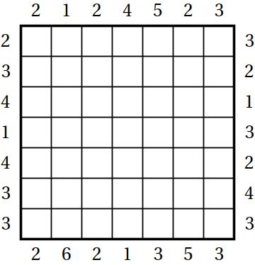
In mathematical terminology we are asked to build a Latin square such that each row is a permutation of length n with a given number of left-to-right and right-to-left-maxima. The following 7 by 7 puzzle is from the Eighth World Puzzle Championship.
Latin squares are notoriously complicated and difficult to understand, so instead of asking about the entire puzzle we discuss the mathematics of a single row. What can you say about a row if you ignore all other info? First of all, let us tell you that the numbers outside have to be between 1 and n. The sum of the left and the right numbers needs to be between 3 and n+1. We leave the proof as an exercise.
Let’s continue with the simplest case. Suppose the two numbers are n and 1. In this case, the row is completely defined. There is only one possibility: the buildings should be arranged in the increasing order from the side where we see all of them.
Now we come to the question we are interested in. Given the two outside numbers, how many permutations of the buildings are possible? Suppose the grid size is n and the outside numbers are a and b. Let’s denote the total number of permutations by fn(a, b). We will assume that a is on the left and b is on the right.
In a previous example, we showed that fn(n, 1) = 1. And of course we have fn(a, b) = fn(b, a).
Let’s discuss a couple of other examples.
First we want to discuss the case when the sum of the border numbers is the smallest — 3. In this case, fn(1, 2) is (n−2)!. Indeed, we need to put the tallest building on the left and the second tallest on the right. After that we can permute the leftover buildings anyway we want.
Secondly we want to discuss the case when the sum of the border numbers is the largest — n+1. In this case fn(a,n+1-a) is (n-1) choose (a-1). Indeed, the position of the tallest building is uniquely defined — it has to take the a-th spot from the left. After that we can pick a set of a-1 buildings that go to the left from the tallest building and the position is uniquely defined by this set.
Before going further let us see what happens if only one of the maxima is given. Let us denote by gn(a) the number of permutations of n buildings so that you can see a buildings from the left. If we put the shortest building on the left then the leftover buildings need to be arrange so that you can see a-1 of them. If the shortest building is not on the left, then it can be in any of the n-1 places and we still need to rearrange the leftover buildings so that we can see a of them. We just proved that the function gn(a) satisfies the recurrence:

Actually gn(a) is a well-known function. The numbers gn(a) are called unsigned Stirling numbers of the first kind (see https://oeis.org/A132393); not only do they count permutations with a given number of left-to-right (or right-to-left) maxima, but they also count permutations with a given number of cycles, and they appear as the coefficients in the product (x + 1)(x + 2)(x + 3)…(x + n), among other places. (Another pair of exercises.)
We are now equipped to calculate fn(1, b). The tallest building must be on the left, and the rest could be arranged so that, in addition to the tallest building, b-1 more buildings are seen from the right. That is fn(1, b) = gn-1(b-1).
Here is the table of non-zero values of fn(1, b).
| b=2 | b=3 | b=4 | b=5 | b=6 | b=7 | |
|---|---|---|---|---|---|---|
| n=2 | 1 | |||||
| n=3 | 1 | 1 | ||||
| n=4 | 2 | 3 | 1 | |||
| n=5 | 6 | 11 | 6 | 1 | ||
| n=6 | 24 | 50 | 35 | 10 | 1 | |
| n=7 | 120 | 274 | 225 | 85 | 15 | 1 |
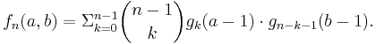
Now we have everything we need to consider the general case. In any permutation of length n, the left-to-right maxima consist of n and all left-to-right maxima that lie to its left; similarly, the right-to-left maxima consist of n and all the right-to-left maxima to its right. We can take any permutation counted by fn(a, b) and split it into two parts: if the value n is in position k + 1 for some 0 ≤ k ≤ n-1, the first k values form a permutation with a – 1 left-to-right maxima and the last n – k – 1 values form a permutation with b – 1 right-to-left maxima, and there are no other restrictions. Thus:
Let’s have a table for f7(a,b), of which we already calculated the first row:
| b=1 | b=2 | b=3 | b=4 | b=5 | b=6 | b=7 | |
|---|---|---|---|---|---|---|---|
| a=1 | 0 | 120 | 274 | 225 | 85 | 15 | 1 |
| a=2 | 120 | 548 | 675 | 340 | 75 | 6 | 0 |
| a=3 | 274 | 675 | 510 | 150 | 15 | 0 | 0 |
| a=4 | 225 | 340 | 150 | 20 | 0 | 0 | 0 |
| a=5 | 85 | 75 | 15 | 0 | 0 | 0 | 0 |
| a=6 | 15 | 6 | 0 | 0 | 0 | 0 | 0 |
| a=7 | 1 | 0 | 0 | 0 | 0 | 0 | 0 |
We see that the first two rows of the puzzle above correspond to the worst case. If we ignore all other constrains there are 675 ways to fill in each of the first two rows. By the way, the sequence of the number of ways to fill in the most difficult row for n from 1 to 10 is: 1, 1, 2, 6, 22, 105, 675, 4872, 40614, 403704. The maximizing pairs (a,b) are (1, 1), (1, 2), (2, 2), (2, 2), (2, 2), (2, 3), (2, 3), (2, 3), (3, 3).
The actual skyscraper puzzles are designed so that they have a unique solution. It is the interplay between rows and columns that allows to reduce the number of overall solutions to one.
Share: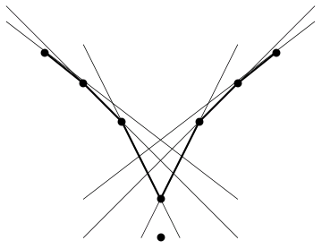
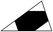
 Sid Dhawan was one of our RSI 2011 math students. He was studying interlocking polyominoes under the mentorship of