Tanya Khovanova's Math Blog

I have two admirers, Alex and Mike. Alex lives next to my home and Mike lives next to my MIT office. I have a lousy memory, so I invented the following system to guarantee that I see both of my friends and also manage to come to my office from time to time. I have a sign hanging on the inside of my home door that says Office on one side and Alex on the other. When I approach the door, I can see right away where I went last time. So I flip the sign and that tells me where next to go. I have a similar sign inside my office door that tells me to go either to home or to Mike. Every evening I spend with one of my admirers discussing puzzles or having coffee. Late at night I come home to sleep in my own bed. Now let’s see what happens if today my home sign shows Office and the office sign shows Mike:

• Today. I flip the home sign to Alex and spend the evening with Alex.
• Tomorrow. I flip the home sign to Office and go to MIT. Later I flip the office sign to Home and return home. As I cannot stand to spend the evening at home alone, I go out again. I flip the home sign to Alex and spend the evening with Alex.
• The day after tomorrow. I flip the home sign to Office and go there. Later I flip the office sign to Mike and spend the evening with Mike.

After three days the signs return to their original positions, meaning that the situation is periodic and I will repeat this three-day pattern forever.

Let’s get back to reality. I am neither memory-challenged nor addicted to coffee. I invented Alex and Mike to illustrate a rotor-router network. In general my home is called a source: the place where I wake up and start the day. There can only be one source in the network. My admirers are called targets and I can have an infinite number of them. The network needs to be constructed in such a way that I always end up with a friend by the end of the day. There could be many other places that I can visit, other than my office: for example, the library, the gym, opera and so on. These places are other vertices of a network that could be very elaborate. Any place where I go, there is a sign that describes a pattern of where I go from there. The sign is called a rotor.

The patterns at every rotor might be more complicated than a simple sign. Those patterns are called rotor types. My sign is called 12 rotor type as it switches between the first and the second directions at every non-friend place I visit.

The sequence of admirers that I visit is called a hitting sequence and it can be proved that the sequence is eventually periodic. Surprisingly, the stronger result is also true: the hitting sequence is purely periodic.

The simple 12 rotor is universal. That means that given a set of friends and a fancy periodic schedule that designates the order I want to visit them in, I can create a network of my activities where every place has a sign of this type 12 and where I will end up visiting my friends according to my pre-determined periodic schedule.

It is possible to see that not every rotor type is universal. For example, palindromic rotor types generate only palindromic hitting sequences, thus they are not universal. The smallest such example, is rotor type 121. Also, block-repetitive rotor types, like 1122, generate block-repetitive hitting sequences.

It is a difficult and an interesting question to describe universal rotor types. My PRIMES student Xiaoyu He was given a project, suggested by James Propp, to prove or disprove the universality of the 11122 rotor type. This was the smallest rotor type the universality of which was not known. Xiaoyu He proved that 11122 is universal and discovered many other universal rotor types. His calculations support the conjecture that only palindromic or block-repetitive types are not universal. You can find these results and many more in his paper: On the Classification of Universal Rotor-Routers.

Recently I stumbled on a cute xkcd comic with the hidden message:

Wikipedia trivia: if you take any article, click on the first link in the article text not in parentheses or italics, and then repeat, you will eventually end up at “Philosophy”.

Naturally, I started to experiment. The first thing I tried was mathematics. Here is the path: Mathematics — Quantity — Property — Modern philosophy — Philosophy.

Then I tried physics, which led me to mathematics: Physics — Natural science — Science — Knowledge — Fact — Information — Sequence — Mathematics.

Then I tried Pierre de Fermat, who for some strange reason led to physics first: Pierre de Fermat — French — France — Unitary state — Sovereign state — State — Social sciences — List of academic disciplines — Academia — Community — Living — Life — Objects — Physics.

The natural question is: what about philosophy? Yes, philosophy goes in a cycle: Philosophy — Reason — Rationality — philosophy.

The original comic talks about spark plugs. So I tried that and arrived at physics: Spark plug — Cylinder head — Internal combustion engine — Engine — Machine — Machine (mechanical) — Mechanical system — Power — Physics.

Then I tried to get far away from philosophy and attempted sex, unsuccessfully: Sex — Biology — Natural science. Then I tried dance: Dance — Art — Sense — Physiology — Science.

It is interesting to see how many steps it takes to get to philosophy. Here is the table for the words I tried:

Mathematics wins. It thoroughly beats all the other words I tried. For now. Fans of sex might be disappointed by these results, and tomorrow they might change the wiki essay about sex to start as:

Modern philosophy considers sex …

I recently stumbled upon some notes (in Russian) of a public lecture given by Vladimir Arnold in 2006. In this lecture Arnold defines a notion of complexity for finite binary strings.

Consider a set of binary strings of length n. Let us first define the Ducci map acting on this set. The result of this operator acting on a string a₁a₂…a_n is a string of length n such that its i-th character is |a_i − a_(i+1)| for i < n, and the n-th character is |a_n − a₁|. We can view this as a difference operator in the field F₂, and we consider strings wrapped around. Or we can say that strings are periodic and infinite in both directions.

Let’s consider as an example the action of the Ducci map on strings of length 6. Since the Ducci map respects cyclic permutation as well as reflection, I will only check strings up to cyclic permutation and reflection. If I denote the Ducci map as D, then the Ducci operator is determined by its action on the following 13 strings, which represent all 64 strings up to cyclic permutation and reflection: D(000000) = 000000, D(000001) = 000011, D(000011) = 000101, D(000101) = 001111, D(000111) = 001001, D(001001) = 011011, D(001011) = 011101, D(001111) = 010001, D(010101) = 111111, D(010111) = 111101, D(011011) = 101101, D(011111) = 100001, D(111111) = 000000.

Now suppose we take a string and apply the Ducci map several times. Because of the pigeonhole principle, this procedure is eventually periodic. On strings of length 6, there are 4 cycles. One cycle of length 1 consists of the string 000000. One cycle of length 3 consists of the strings 011011, 101101 and 110110. Finally, there are two cycles of length 6: the first one is 000101, 001111, 010001, 110011, 010100, 111100, and the second one is shifted by one character.

We can represent the strings as vertices and the Ducci map as a collection of directed edges between vertices. All 64 vertices corresponding to strings of length 6 generate a graph with 4 connected components, each of which contains a unique cycle.

The Ducci map is similar to a differential operator. Hence, sequences that end up at the point 000000 are similar to polynomials. Arnold decided that polynomials should have lower complexity than other functions. I do not completely agree with that decision; I don’t have a good explanation for it. In any case, he proposes the following notion of complexity for such strings.

Strings that end up at cycles of longer length should be considered more complex than strings that end up at cycles with shorter length. Within the connected component, the strings that are further away from the cycle should have greater complexity. Thus the string 000000 has the lowest complexity, followed by the string 111111, as D(111111) = 000000. Next in increasing complexity are the strings 010101 and 101010. At this point the strings that represent polynomials are exhausted and the next more complex strings would be the three strings that form a cycle of length three: 011011, 101101 and 110110. If we assign 000000 a complexity of 1, then we can assign a number representing complexity to any other string. For example, the string 111111 would have complexity 2, and strings 010101 and 101010 would have complexity 3.

I am not completely satisfied with Arnold’s notion of complexity. First, as I mentioned before, I think that some high-degree polynomials are so much uglier than other functions that there is no reason to consider them having lower complexity. Second, I want to give a definition of complexity for periodic strings. There is a slight difference between periodic strings and finite strings that are wrapped around. Indeed, the string 110 of length 3 and the string 110110 of length 6 correspond to the same periodic string, but as finite strings it might make sense to think of string 110110 as more complex than string 110. As I want to define complexity for periodic strings, I want the complexity of the periodic strings corresponding to 110 and 110110 to be the same. So this is my definition of complexity for periodic strings: let’s call the complexity of the string the number of edges we need to traverse in the Ducci graph until we get to a string we saw before. For example, let us start with string 011010. Arrows represent the Ducci map: 011010 → 101110 → 110011 → 010100 → 111100 → 000101 → 001111 → 010001 → 110011. We saw 110011 before, so the number of edges, and thus the complexity, is 8.

The table below describes the complexity of the binary strings of length 6. The first column shows one string in a class up to a rotation or reflections. The second column shows the number of strings in a class. The next column provides the Ducci map of the given string, followed by the length of the cycle. The last two columns show Arnold’s complexity and my complexity.

As you can see, for examples of length six my complexity doesn’t differ much from Arnold’s complexity, but for longer strings the difference will be more significant. Also, I am pleased to see that the sequence 011010, the one that I called The Random Sequence in one of my previous essays, has the highest complexity.

I know that my definition of complexity is only for periodic sequences. For example, the binary expansion of pi will have a very high complexity, though it can be represented by one Greek letter. But for periodic strings it always gives a number that can be used as a measure of complexity.

The last time I talked to John H. Conway, he taught me to walk up the stairs. It’s not that I didn’t know how to do that, but he reminded me that a nerd’s goal in climbing the steps is to establish the number of steps at the end of the flight. Since it is boring to just count the stairs, we’re lucky to have John’s fun system.

His invention is simple. Your steps should be in a cycle: short, long, long. Long in this case means a double step. Thus, you will cover five stairs in one short-long-long cycle. In addition, you should always start the first cycle on the same foot. Suppose you start on the left foot, then after two cycles you are back on the left foot, having covered ten stairs. While you are walking the stairs in this way, it is clear where you are in the cycle. By the end of the staircase, you will know the number of stairs modulo ten. Usually there are not a lot of stairs in a staircase, so you can easily estimate the total if you know the last digit of that number.

I guess I am not a true nerd. I have lived in my apartment for eight years and have never bothered to count the number of steps. That is, until now. Having climbed my staircase using John’s method, I now know that the ominous total is 13. Oh dear.

Lionel Levine invented a new hat puzzle.

The sultan decides to torture his hundred wise men again. He has an unlimited supply of red and blue hats. Tomorrow he will pile an infinite, randomly-colored sequence of hats on each wise man’s head. Each wise man will be able to see the colors of everyone else’s hats, but will not be able to see the colors of his own hats. The wise men are not allowed to pass any information to each other.
At the sultan’s signal each has to write a natural number. The sultan will then check the color of the hat that corresponds to that number in the pile of hats. For example, if the wise man writes down “four,” the sultan will check the color of the fourth hat in that man’s pile. If any of the numbers correspond to a red hat, all the wise men will have their heads chopped off along with their hats. The numbers must correspond to blue hats. What should be their strategy to maximize their chance of survival?

Suppose each wise man writes “one.” The first hat in each pile is blue with a probability of one-half. Hence, they will survive as a group with a probability of 1 over 2¹⁰⁰. Wise men are so wise that they can do much better than that. Can you figure it out?

Inspired by Lionel, I decided to suggest the following variation:

This time the sultan puts two hats randomly on each wise man’s head. Each wise man will see the colors of other people’s hats, but not the colors of his own. The men are not allowed to pass any info to each other. At the sultan’s signal each has to write the number of blue hats on his head. If they are all correct, all of them survive. If at least one of them is wrong, all of them die. What should be their strategy to maximize their chance of survival?

Suppose there is only one wise man. It is clear that he should write that he has exactly one blue hat. He survives with the probability of one-half. Suppose now that there are two wise men. Each of them can write “one.” With this strategy, they will survive with a probability of 1/4. Can they do better than that? What can you suggest if, instead of two, there is any number of wise men?

86 is conjectured to be the largest power of 2 not containing a zero. This simply stated conjecture has proven itself to be proof-resistant. Let us see why.

What is the probability that the nth power of two will not have any zeroes? The first and the last digits are non-zeroes; suppose that other digits become zeroes randomly and independently of each other. This supposition allows us to estimate the probability of 2ⁿ not having zeroes as (9/10)^k-2, where k is the number of digits of 2ⁿ. The number of digits can be estimated as n log₁₀2. Thus, the probability is about cxⁿ, where c = (10/9)² ≈ 1.2 and x = (9/10)^log₁₀2 ≈ 0.97. The expected number of powers of 2 without zeroes starting from the power N is cx^N/(1-x) ≈ 40 ⋅ 0.97^N.

Let us look at A007377, the sequence of numbers such that their powers of 2 do not contain zeros: 1, 2, 3, 4, 5, 6, 7, 8, 9, 13, 14, 15, 16, 18, 19, 24, 25, 27, 28, 31, 32, 33, 34, 35, 36, 37, 39, 49, 51, 67, 72, 76, 77, 81, 86. Our estimates predicts 32 members of this sequence starting from 6. In fact, the sequence has 30 conjectured members. Similarly, our estimate predicts 2.5 members starting from 86. It is easy to check that the sequence doesn’t contain any more numbers below 200 and our estimate predicts 0.07 members after 200. As we continue checking larger numbers and see that they do not belong to the sequence, the probability that the sequence contains more elements vanishes. With time we check more numbers and become more convinced that the conjecture is true. Currently, it has been checked up to the power 4.6 ⋅ 10⁷. The probability of finding something after that is about 1.764342396 ⋅10^-633620.

Let us try to approach the conjecture from another angle. Let us check the last K digits of powers of two. As the number of possibilities is finite, these last digits eventually will start cycling. If we can show that all the elements inside the period contain zeroes, then we need to check the finite number of powers of two until this period starts. If we can find such K, we can prove the conjecture.

Let us look at the last two digits of powers of two. The sequence starts as: 01, 02, 04, 08, 16, 32, 64, 28, 56, 12, 24, 48, 96, 92, 84, 68, 36, 72, 44, 88, 76, 52, 04. As we would anticipate, it starts cycling. The cycle length is 20, and 90% of numbers in the cycle don’t have zeroes.

Now let’s continue to the last three digits. The period length is 100, and 19 of them either start with zero or contain zero. The percentage of elements in the cycle that do not contain zero is 81%.

The cycle length for the last n digits is known. It is 4 ⋅ 5^n-1. In particular the cycle length grows by 5 every time. The number of zero-free elements in these cycles form a sequence A181610: 4, 18, 81, 364, 1638, 7371, 33170. If we continue with our supposition that the digits are random, and study the new digits that appear when we move from the cycle of the last n digits to the next cycle of the last n+1 digits, we can expect that 9/10 of those digits will be non-zero. Indeed, if we check the ratio of how many numbers do not contain zero in the next cycle compared to the previous cycle, we get: 4.5, 4.5, 4.49383, 4.5, 4.5, 4.50007. All of these numbers are quite close to our estimation of 4.5. If this trend continues the portion of the numbers in the cycle that don’t have zeroes tends to zero; however, the total of such numbers grows exponentially. We can even estimate that the expected growth is 4 ⋅ 4.5^n-1. From this estimation, we can derive the conjecture:

Conjecture. For any number N, there exists a power of two such that its last N digits are zero-free.

Indeed, the last N digits of powers of two cycle, and there are an increasing number of members inside that cycle that do not contain zeroes. The corresponding powers of two don’t have zeroes among N rightmost digits.

So, how do we combine the two results? First, the expected probability of finding the power of two larger than 86 that doesn’t contain zero is minuscule. And second, we most certainly can find a power of two that has as many zeroless digits at the end as we want.

To combine the two results, let us look at the sequences A031140 and A031141. We can deduce from them that for the power 103233492954 the first zero from the right occupies the 250th spot. The total number of digits of that power is 31076377936. So 250 is a tiny portion of the digits.

As time goes by we grow more and more convinced that 86 is the largest power of two without zeroes, but it is not at all clear how we can prove the conjecture or whether it can be proven at all.

My son, Sergei, suggested that I claim that I have a proof of this conjecture, but do not have enough space in the margin to fit my proof in. The probability that I will ever be shamed and disproven is lower than the probability of me winning a billion dollars in the lottery. Though then, if I do win the big bucks, I will still care about being shamed and disproven.

Once again I am one of the organizers of the Women and Math Program at the Institute for Advanced Study in Princeton, May 16-27, 2011. It will be devoted to an exciting modern subject: Sparsity and Computation.

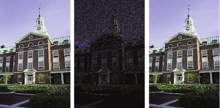
In case you are wondering about the meaning of the picture on the program’s poster (which I reproduce below), let us explain.

The left image is the original picture of Fuld Hall, the main building on the IAS campus. The middle image is a corrupted version, in which you barely see anything. The right image is a striking example of how much of the image can be reconstructed from the corrupted image using clever algorithms.

Female undergraduates, graduates and postdocs are welcome to apply to the program. You will learn exactly how the corrupted image was recovered and much more. The application deadline is February 20, 2011.

Eugene Brevdo generated the pictures for our poster and agreed to write a piece for my blog explaining how it works. I am glad that he draws parallels to food, as the IAS cafeteria is one of the best around.

by Eugene Brevdo

The three images you are looking at are composed of pixels. Each pixel is represented by three integers corresponding to red, green, and blue. The values of each integer range between 0 and 255.

The image of Fuld hall has been corrupted: some pixels have been replaced with all 0s, and are therefore black; this means the pixel was not “observed”. In this corrupted version, 85% of the pixel values were not observed. Other pixels have been modified to various degrees by stationary Gaussian noise (i.e. independent random noise). For the 15% observed pixel values, the PSNR is 6.5 db. As you can see, this is a badly corrupted image!

The really interesting image is the one on the right. It is a “denoised” and “inpainted” version of the center image. That means the pixels that were missing were filled in and the observed pixel integer values were re-estimated. The algorithm that performed this task, with the longwinded name “Nonparametric Bayesian Dictionary Learning,” had no prior knowledge about what “images should look like”. In that sense, it’s similar to popular wavelet-based denoising techniques: it does not need a prior database of images to correct a new one. It “learns” what parts of the image should look like from the original image, and fills them in.

Here’s a rough sketch of how it works. The idea is to use a new technique in probability theory — the idea that a a patch, e.g. a contiguous subset of pixels, of an image is composed of a sparse set of basic texture atoms (from the “Dictionary”). Unfortunately for us, the number of atoms and the atoms themselves are unknowns and need to be estimated (the “Nonparametric Learning” part). In a way, the main idea here is very similar to Wavelet-based estimation, because while Wavelets form a fixed dictionary, a patch from most natural images is composed of only a few Wavelet atoms; and Wavelet denoising is based on this idea.

We make two assumptions that allow us to simplify and solve this problem, which is unwieldy-sounding and vague when the texture atoms have to be estimated. First, there may be many atoms, but a single patch is a combination of only a sparse subset of them. Second, because each atom appears in part in many patches, even if we observe some noisily, once we know which atoms appear in which patches, we can invert and average together all of the patches associated with an atom to estimate it.

To explain and programmatically implement the full algorithm that solves this problem, probability theorists like to explain things in terms of going to a buffet. Here’s a very rough idea. There’s a buffet with a (possibly infinite) number of dishes. Each dish represents a texture atom. An image patch will come up to the buffet and, starting from the first dish, begins to flip a biased coin. If the coin lands on heads, the patch takes a random amount of food from the dish in front of it (the atom-patch weight), and then walks to the next dish. If the coin lands on tails, the patch skips that dish and instead just walks to the next. There it flips its coin with a different bias and repeats the process. The coins are biased so the patch only eats a few dishes (there are so many!). When all is said and done, however, the patch has eaten a random amount from a few dishes. Rephrased: the image patch is made from a weighted linear combination of basic atoms.

At the end of the day, all the patches eat their own home-cooked dessert that didn’t come from the buffet (noise), and some pass out from eating too much (missing pixels).

If we know how much of each dish (texture atom) each of the patches ate and the biases of the coins, we can estimate the dishes themselves — because we can see the noisy patches. Vice versa, if we know what the dishes (textures) are, and what the patches look like, we can estimate the biases of the coins and how much of a dish each patch ate.

At first we take completely random guesses about what the dishes look like and what the coins are, as well as how much each patch ate. But soon we start alternating guesses between what the dishes are, the coin biases, and the amounts that each patch ate. And each time we only update our estimate of one of these unknowns, on the assumption that our previous estimates for the others is the truth. This is called Gibbs sampling. By iterating our estimates, we can build up a pretty good estimate of all of the unknowns: the texture atoms, coin biases, and the atom-patch weights.

The image on the right is our best final guess, after iterating this game, as to what the patches look like after eating their dishes, but before eating dessert and/or passing out.

Silvio Micali taught me cryptography. To explain one-way functions, he gave the following example of encryption. Alice and Bob procure the same edition of the white pages book for a particular town, say Cambridge. For each letter Alice wants to encrypt, she finds a person in the book whose last name starts with this letter and uses his/her phone number as the encryption of that letter.

To decrypt the message Bob has to read through the whole book to find all the numbers. The decryption will take a lot more time than the encryption. If the book increases in size the time it takes Alice to do the encryption almost doesn’t increase, but the decryption process becomes more and more draining.

This example is very good for teaching one-way functions to non-mathematicians. Unfortunately, the technology changes and the example that Micali taught me fifteen years ago isn’t so cute anymore. Indeed you can do a reverse look-up online of every phone number in the white pages.

I still use this example, with an assumption that there is no reverse look-up. I recently taught it to my AMSA students. And one of my 8th graders said, “If I were Bob, I would just call all the phone numbers and ask their last names.”

In the fifteen years since I’ve been using this example, this idea never occurred to me. I am very shy so it would never enter my mind to call a stranger and ask for their last name. My student made me realize that my own personality affected my mathematical inventiveness.

Since modern technology is murdering my 15-year-old example, I would like to ask my readers to suggest other simple examples of one-way functions or ways to resurrect the white pages example.

I asked my son Alexey Radul what exactly he is doing for his postdoc at the Hamilton Institute in Ireland. Here is his reply:

The short, jargon-loaded version: We are building an optimizing compiler for a programming language with first-class automatic differentiation, and exploring mathematical foundations, connections, applications, etc.

Interpretation of jargon:

Automatic differentiation is a technique for turning a program that computes a function into a program that computes that function together with its derivative; with a constant factor overhead. This is better than the usual symbolic differentiation that, say, Mathematica does because there is no intermediate-expression bulge. For example, if your function is a large product

Product f1(x) f2(x) … fn(x),

the symbolic derivative has size n²

Sum (Product f1′(x) f2(x) … fn(x)) (Product f1(x) f2′(x) … fn(x)) … (Product f1(x) f2(x) … fn'(x))

automatic differentiation avoids that cost. Automatic (as opposed to symbolic) differentiation also extends to conditionals, data structures, higher-order functions, and all the other wonderful things that distinguish a computer program from a mathematical expression.

First-class means that the differentiation operations are normal citizens of the programming language. This is not the case with commonly used automatic differentiation systems, which are all preprocessors that rewrite C or Fortran source code. In particular, we want to be able to differentiate any function written in the language, even if it is a derivative of something, or contains a derivative of something, etc. The automatic differentiation technique works but becomes more complicated in the presence of higher order, multivariate, or nested derivatives.

We are building an optimizing compiler because the techniques necessary to get good performance and correct results with completely general automatic differentiation are exactly the techniques used to produce aggressive optimizing compilers for functional languages, so we might as well go all the way.

It appears that the AD trick (or at least half of it) is just an implementation of synthetic differential geometry in the computer. This leads one to hope that a good mathematical foundation can be found that dictates the behavior of the system in all the interesting special cases; there is lots of math to be thought about in the vicinity of this stuff.

Applications are also plentiful. Any time you want to optimize anything with respect to real parameters, gradients help. Any time you are dealing with curves, slopes help. Computer graphics, computer vision, physics simulations, economic and financial models, probabilities — there’s so much stuff to apply a high quality such system to that we don’t know where to begin.

Fifteen years ago I attended Silvio Micali‘s cryptography course. During one of the lectures, he asked me to close my eyes. When I did, he wrote a random sequence of coin flips of length six on the board and invited me to guess it.

I am a teacher at heart, so I imagined a random sequence I would write for my students. Suppose I start with 0. I will not continue with zero, because 00 looks like a constant sequence, which is not random enough. So my next step would be sequence 01. For the next character I wouldn’t say zero, because 010 seems to promise a repetitive pattern 010101. So my next step would be 011. After that I do not want to say one, because I will have too many ones. So I would follow up with 0110. I need only two more characters. I do not want to end this with 11, because the result would be periodic, I do not want to end this with 00, because I would have too many zeroes. I do not want to end this with 01, because the sequence 011001 has a symmetry: reversing and negating this sequence produces the same sequence.

During the lecture all these considerations happened in the blink of an eye in my mind. I just said: 011010. I opened my eyes and saw that Micali had written HTTHTH on the board. He was not amused and may even have thought that I was cheating.

Many teachers, when writing a random sequence, do not flip a coin. They choose a sequence that looks “random”: it doesn’t have too many repetitions and the number of ones and zeroes is balanced (that is, approximately the same). When they write it character by character on the board, they often choose a sequence so that any prefix looks “random” too.

As a result, the sequence they choose stops being random. Actually, they’re making a choice from a small set of sequences that look “random”. So the fact that I guessed Micali’s sequence is not surprising at all.

If you have gone to many math classes, you’ve seen a lot of professors choosing very similar-looking “random” sequences. This discriminates against sequences that do not look “random”. To restore fairness to those under-represented sequences, I have decided that the next time I need a random sequence, I will choose 000000.